Francesco Caravenna

PhD course, Spring 2014

Random Graphs and Complex Networks

Federico Bassetti and Francesco Caravenna

Presentation

This course is an introduction to the mathematical modeling of random graphs.

Only a basic probabilistic background is required (finite and countable probability, discrete random variables), making the course accessible to every mathematical student. One of our aims is to illustrate some interesting ideas and techniques of modern probability theory in an accessible and relatively non-technical framework.

Here are some slides presenting the course.

Summary

In recent years there has been an increasing interest for real-world networks, such as the internet, collaboration and citation networks, social relations, biological and ecological networks. A remarkable fact is that such different examples show surprisingly similar large-scale features. For instance, these networks are "small worlds", meaning that typical distances among nodes grow slowly with the size of the network, and many of them are "scale free", meaning that the empirical distribution of the degrees (number of nodes connected to a given node) is almost independent of the size of the network, and shows a power-law decay. In order to explain such features, many efforts have been devoted to the study of mathematical models that go under the name of "random graphs".

One of the simplest way to produce a random graph, having {1, 2, ..., n} as the sets of nodes, is to toss a coin for each couple (i,j) of nodes, putting a connection between them if a head comes up (the coins are assumed to be independent, and to give head with the same probability p). This model was investigated already in the late 1950s by Erdos and Renyi, who showed that an interesting "phase transition" occurs: depending on how the probability p scales with n, the graph either presents a "giant connected component", of size proportional to n, or it consists of many "small disconnected ilands", of size at most log(n). Despite its apparent simplicity, the fine properties of this model are far from trivial and are amenable to a thorough mathematical analysis. This will be the main object of the first part of the course.

The Erdos-Renyi random graph is not a good model for many real-world networks, because it is not scale free. For this reason, in the last decades several alternative models have been proposed and investigated. We will focus on two of the most popular ones: the "configuration model", a random graph model in which the degrees are fixed beforehand and the nodes are connected in the most random way, and the "preferential attachment model", where the graph is built dynamically, adding nodes to the network in a sequential fashion, favoring connections among nodes with large degrees. Both classes of models lead to scale free and small world networks and one can prove precise asymptotic results for the typical distances and degree distributions. This will be the object of the second part of the course.

References

• The course will be mainly based on the lecture notes Random Graphs and Complex Networks by Remco van der Hofstad, available on the author webpage.
• Another relevant reference is the book Random Graph Dynamics by Rick Durrett, Cambridge Unversity Press (2006) (see here for more information).

Tentative Program

1. Probabilistic Tools and Techniques: random variables, coupling, inequalities.
2. Branching Processes as Random Trees: asymptotic properties.
3. The Erdos-Renyi Random Graph: phase transition and giant component.
4. Configuration Model: asymptotic distances and small world phenomenon.
5. Preferential Attachment: emergence of a scale free network.

Lectures Log

References:

• [vdH] R. van der Hostad Random graphs and complex networks, lecture notes available on the author webpage
• [LP] R. Lyons, Y. Peres. Probability on Trees and Networks, available here
• [CDP] Caravenna, Dai Pra. Probabilità: Un'introduzione attraverso modelli e applicazioni. Springer.

Lecture 10 (27th May 2014)

• Preferential attachment model.
  • Reminders of definition and Markov property of degree (D_i(t))_{t ∈ N}.
  • Remark: if E[Y_t | F_t-1] = (η_t-1) Y_t-1 and Y₀ = y₀, for some constants η_t > 1 and y₀ > 0, the process M_t := (∏ _{s ≤ t-1} 1/η_s) Y_t / y₀ is a martingale. Corollary: D_i(t) / t^1/(2+δ) is bounded in L² [exercise: considering Y_t := (D_i(t) + δ) (D_i(t) + δ + 1)].
• Azuma-Hoeffding inequality for martingales with bounded increments: discussion and proof (Thm 2.24 [vdH]).
• Asymptotic properties of degrees in the preferential attachment model.
  • Concentration of N_k(t) (number of vertexes of degree k) around its expected value, using the Azuma-Hoeffding inequality (Prop 8.3 [vdH]).
  • Detailed proof that (M_n := E[N_k(t) | F_n])_{n ∈ N} is a martingale with bounded increments (|M_n - M_n-1| ≤ 2) using the Markov property of (D_i(t))_{t ∈ N}.
  • Asymptotic behavior of E[N_k(t)] ∼ t p_k with p_k ∼ c_δ / k^3+δ using recursive equations (Prop. 8.4 [vdH], sketch of the proof).

Lecture 9 (20th May 2014)

• Preferential attachment model.
  • Motivation and introduction to the model.
  • PA(t) = PA^(1,δ)(t) defined as a function of the sequence of random variables Z_i ∈ {1, ..., i}, for i=1, ..., t, where Z_i is the vertex to which the vertex "i" is attached. Distribution of the random variables Z_i's.
  • σ-algebra F_t and its interpretation. The process (D_i(t))_{t ∈ N}, giving the degree of a vertex "i" as a function of t, is a Markov chain.
  • Extension of the model: PA^(m,δ)(t) for m ≥ 2 in terms of PA^(1,δ/m)(mt).
• Asymptotic properties of degrees in the preferential attachment model.
  • Empirical degree distribution in PA(t) as a random probability on N, which converges to a heavy-tailed distribution (Thm 8.2 [vdH], proof next time).
  • Reminders on martingales, conditions for a.s. and L^p convergence.
  • Reminders on Euler's Gamma function Γ(t).
  • Degrees of fixed vertices: expected value and asymptotic behavior of D_i(t) as t → ∞ (Thm. 8.1 [vdH]).
  • Heuristic derivation of heavy tails for the empirical degree distribution from the knowledge E[D_i(t)] ∼ c (t/i)^1/(τ-1) (with τ = 3+δ).

Lecture 8 (13th May 2014)

• Size biasing: discussion and examples.
• Phase transition in the configuration model, revisited.
  • Emergence of a giant component according to whether ν > 1 or ν ≤ 1, where ν := E[D(D-1)]/E[D] (Thm 10.1 [vdH], no proof).
  • Heuristics: two-stage branching process with size-biased distribution.
• Polynomial τ-condition (with τ ∈ (2,3)) for a sequence d⁽ⁿ⁾ = (d₁⁽ⁿ⁾, ..., d_n⁽ⁿ⁾).
• Small world phenomenon in the configuration model:
  • log log n asymptotic behavior for the diameter of the configuration model with heavy tails (polynomial τ-condition): (Theorem 10.33 [VdH]; partial proof of the upper bound, see below).
  • Proposition 1: log log n upper bound on the diameter of the Core (Theorem 10.28 [VdH], no proof).
  • Proposition 2: log log n upper bound on the distance from the Core (proof as a consequence of Propositions 3 and 4 below).
  • Proposition 3: estimate on the connection probability of two subsets of vertices (enhanced version of Lemma 10.30 [VdH], with proof).
  • Proposition 4: estimate on the "effective degree" (number of half-edges) of the neighborhood N_≤k(v) of a vertex v (sketch of the proof).

Lecture 7 (6th May 2014)

• Proof of the convergence of the empirical degree distribution p_k^ER,(n) of the erased configuration model CM_n^ER(d) (Thm 7.6 [vdH]).
  • Pointwise convergence p_k⁽ⁿ⁾ → p_k for every fixed k is equivalent to ℓ¹ convergence ∑_k |p_k⁽ⁿ⁾ - p_k| → 0.
  • If α_n → ∞, the fraction of vertexes v ∈ [n] with d_v > α_n vanishes.
  • Estimate of ∑_k |p_k^ER,(n) - p_k⁽ⁿ⁾| in terms of the fraction of vertexes v ∈ [n] having at least a self-loop or a multiple-edge.
  • Expected values of the numbers of self-loops (S_v) and multiple edges (M_v) emanating from a vertex v ∈ [n].
  • Determination of the truncation α_n, assuming max{d_v: v ∈ [n]} = o(n).
  • Conclusion: proof that max{d_v: v ∈ [n]} = o(n) if regularity conditions (a) and (b) are satisfied.
• Configuration model with i.i.d. degrees.
  • An i.i.d. sequence D = (D₁, D₂, ...) satisfies a.s. the regularity condition (a), and also (b) and (c) if E[D₁] < ∞ and E[D₁²] < ∞ respectively.
  • Configuration model with i.i.d. degrees CM_n(D) as a function Ψ(D, W), where W are i.i.d. U(0,1) which generate a uniform configuration.
• Phase transition in the configuration model:
  • Emergence of a giant component according to whether ν > 1 or ν ≤ 1, where ν := E[D(D-1)]/E[D] (Thm 10.1 [vdH], no proof).
  • Heuristics: two-stage branching process with size-biased distribution.

Lecture 6 (29th April 2014)

• Beyond Erdos-Renyi:
  • Reminders: Poisson limit of the empirical degree distribution for Erdos-Renyi (Thm 5.9 [vdH], no proof).
  • How to build a model with (asymptotic) polynomial degree distribution? Introduction to Configuration Model and Preferential Attachment.
• Introduction to the Configuration Model (§7.1 [vdH]):
  • Not every d = (d₁, ..., d_n) is the degree sequence of a graph. Graphs, multigraphs and their matrix notation: spaces G_n and MG_n.
  • Intuitive definition of the Configuration Model CM_n(d) via "uniform matching" of the half-edges attached to each vertex in [n].
  • Notation ℓ_n := d₁ + ... + d_n. Space Conf(ℓ_n) of partitions of [ℓ_n] into pairs ("configurations"). Map φ_{d: Conf(ℓn) → MGn between configurations and multigraphs.}
  • How to generate a r.v. U uniformly distributed on Conf(d) via successive uniform pairings. CM_n(d) has the same law as φ(U).
• Basic properties of the Configuration Model:
  • Distribution of CM_n(d): probability of a given multigraph (Prop 7.4 [vdH]).
  • Corollary: conditionally on the event {CM_n(d) ∈ G_n}, the r.v. CM_n(d) is uniformly distributed on G_n. How to sample a uniform simple graph with given degrees d by repeatedly sampling CM_n(d).
  • Regularity conditions (a), (b), (c) for a sequence d⁽ⁿ⁾ = (d₁⁽ⁿ⁾, ..., d_n⁽ⁿ⁾) with respect to a given probability (p_k)_k∈N0. Probabilistic reformulation.
  • Probability of CM_n(d) being a simple graph (Thm 7.8 [vdH], no proof).
  • Erased configuration model CM_n^ER(d). Convergence of the corresponding erased empirical degree distribution (Thm 7.6 [vdH], proof next time).

Lecture 5 (14th April 2014)

• Proof of the law of large numbers for giant component in the supercritical regime.
  • Concentration of the number of vertices in large clusters (Prop 4.10, Coroll 4.11 [vdH]);
  • The law of the random walk in the exploration process (Prop 4.6 [vdH]);
  • No intermediate clusters (Prop 4.12, Coroll 4.13 [vdH]).
• More on supercritical regime.
  • Duality principle for ER random graphs (Section 4.4.2 [vdH]);
  • Connectivity threshold (Thm 5.5 [vdH], without proof).
• Connected components in the critical window of ER random graphs.
  • Statement of the Aldous theorem (Theorem 5.4 [vdH]).
• Degree sequence.
  • Poisson (uniform) limit of the empirical degree distribution (Thm 5.9 [vdH], without proof).

Lecture 4 (8th April 2014)

• Comparing the connected components of an Erdos-Renyi graph with binomial branching processes.
  • Stochastic domination of the cluster size (thm 4.2 [vdH]);
  • Lower bound on cluster tail (thm 4.3 [vdH]).
• Largest component in the subcritical regime.
  • Upper and lower bounds on largest subcritical component and the law of large numbers (thm 4.4/4.5 [vdH]);
  • Complete proofs of the two bounds (following Sections 4.3.1, 4.3.2, 4.3.3 in [vdH] with minor modifications).
• Supercritical regime.
  • Statements of the law of large numbers and the central limit theorem for giant component (thm 4.8, thm 4.15 [vdH]);
  • Statement of the law of large numbers for the second largest component (Sec. 4.4.2 [vdH]).

Lecture 3 (1st April 2014)

• Random-walk perspective to branching processes.
  • Definition of conjugate pair of off-spring distributions and basic properties (ex. 3.16, 3.17 [vdH]);
  • Duality principle for branching processes (thm 3.7 [vdH]);
  • Cramer's upper bound, Chernoff bound (thm 2.17 [vdH]);
  • Extinction probability with large total progeny (thm 3.8 [vdH]).
• Hitting-time theorem and the total progeny.
  • Hitting-time theorem (thm. 3.14 [vdH]);
  • Law of total progeny (thm 3.13 [vdH]);
  • Individuals with an infinite line of descent (thm. 3.11 [vdH]).
• Binomial and Poisson branching processes.
  • Poisson duality principle (thm 3.15 [vdH]);
  • Total progeny distribution for the Poisson branching process (thm. 3.16 [vdH]);
  • Total variation distance, Strassen theorem, Poisson-Binomial coupling (thm. 2.9, thm 2.10 [vdH], see also Capitolo 4 [CDP]);
  • Poisson and binomial branching processes (thm. 3.16 [vdH]).
• Erdos-Renyi random graph.
  • Exploration process for the connected component of a node (random walk perspective);
  • The size of the connected component as the hitting time of S_t and the law of the X_t's (Sec. 4.1 [vdH]).

Lecture 2 (25th March 2014)

• Brancing process.
  • Extinction vs survival (definition and basic results). Thm 3.1 [vdH].
• The intrinsic Martingale and its limit.
  • Thm 3.3, Thm 3.9, result (3.4.1), Exer.3.19 in [vdH];
  • Kesten-Stigum Theorem and Seneta Theorem (statements without proofs), Thm 3.10 [vdH].
  • Definition of inherited property and Proposition 5.6 and Corollary 5.6 in [LP];
  • Conditioning on extinction, conditioning on survival.
• Bernoulli percolation.
  • Definition of general percolation graph, definition of critical probability.
  • Binomial Galton Watson tree as the percolation graph of an n-ary tree.
  • Erdos-Renyi random graph as the percolation graph of a complete graph.
  • Critical probability in a Galton Watson tree, Prop 5.9 in [LP].
• Total progeny.
  • Definition of Total progeny, thm 3.2 in [vdH].
  • Random-walk perspective to branching processes.
  • Definition of History. Total progeny as hitting time of a random walk. Sec. 3.3 [vdH].

Lecture 1 (18 March 2014)

• Graphs and trees.
  • Basic definitions: edges, nodes, self-loop, directed and undirected graphs, tree, rooted tree. Degree of a node.
  • Ulam-Harris tree, rooted labelled trees and locally finite trees.
• Random graphs and random trees.
  • Definition of (finte) random graph and (finte) random tree.
  • Definition of random tree as a random variable on the space of locally finite trees.
  • Definition of Erdos-Renyi graph (density and different constructions).
  • Binomial distribution of the degree of a node in the Erods-Renyi graph and Poisson limit.
• Galton-Watson tree process.
  • The off-spring distribution and the definition of Galton-Watson tree.
  • Basic properties of independence of the Galton-Watson tree.
  • The number of individuals in the n-th generation (the brancing process Z_n).
• Real words networks and random graphs.
  • The proportion of vertices of degree k in some empirical networks and the study of the degree distribution of a random graph.
  • Power-law decay of the degree distribution, hub and small-words in real words networks.

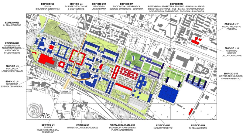
Logistic Details

Due to room shortage, lectures in Milano-Bicocca will take place in different rooms located in different buildings:

• Building U5 is in Via Roberto Cozzi 55
• Building U9 is in Viale dell'Innovazione 10
• Building U7 is in Via Bicocca degli Arcimboldi 8
• Bicocca campus maps: here or here

Schedule for the second part of the course, held in Milano Bicocca:

• Tuesday 29 April 2014, 11:00-12:30 and 14:00-15:30, Aula U5-3014
• Tuesday 6 May 2014, 11:00-12:30 and 14:00-15:30, Aula U9-10
• Tuesday 13 May 2014, 11:00-12:30 and 14:00-15:30, Aula U7-6
• Tuesday 20 May 2014, 11:00-12:30 and 14:00-15:30 14:15-17:30 (with a short break), Aula U7-6
• Tuesday 27 May 2014, 11:00-12:30 and 14:00-15:30, Aula U5-3014

Schedule for the first part of the course, held in Pavia (Dipartimento di Matematica, via Ferrata 1):

• Tuesday 18 March 2014, 11:15-13:15, Aula Beltrami (Introductory Lecture)
• Tuesday 25 March 2014, 11:15-12:45 and 14:00-15:30, Aula C13
• Tuesday 1 April 2014, 11:15-12:45 and 14:00-15:30, Aula Beltrami
• Tuesday 8 April 2014, 11:15-12:45 and 14:00-15:30, Aula Beltrami
• Tuesday 15 April 2014, 11:15-12:45 and 14:00-15:30, Aula Beltrami

Interested students are invited to contact us via email.

What else?

For more information, do not hesitate to contact us via email.